Best Of

Author: Dana Evernden is a Principal Solution Architect at Anaplan, pioneering the Anaplan Delivery Assurance Program.

Polaris Building and Debugging Tactics 

Tired of sluggish models and performance bottlenecks in Polaris? Ever feel like you're just one tweak away from unlocking lightning-fast speed? You've found the link you've always needed. This is your definitive guide to transforming your models from frustratingly slow to incredibly responsive.  

A quick tip for build teams: The most successful, nontroubled projects treat performance tuning as a key part of the process. It’s a small investment that pays huge dividends in the end-user experience, resulting in customer trust that translates to continued implementation phases. Dive into these essential tactics and learn how to build, tune, and debug like a pro, ensuring your end-users get the seamless experience they deserve. 

How to Use This Guide 

• Establish the Foundation: Start with the Key Reminders, When to Use This Guide, and the Performance Checklist. These sections ensure you are applying Polaris best practices at the correct stages of the build lifecycle and within the appropriate model components. 
• Prioritize Impact: When evaluating model performance, follow the Steps for Prioritizing Optimization Opportunities. This section helps you focus on the most impactful metrics first, ensuring your tuning efforts yield the greatest performance gains. 
• Implement Solutions: Consult the Optimization and Debugging Tips for a deep dive into proven methods for refining formulas, reducing engine effort, and resolving common bottlenecks. 

Key Reminders for Building in Polaris 

When building in Polaris, keep these foundational principles in mind: 

• Use ALM from the start: Review this Iterative Development in Polaris community article to properly set up your environments. 
• Monitor metrics closely: Tread carefully and check Calculation Effort, Memory, and Populated Cell Count frequently when building in large, highly dimensionalized modules (e.g., output, reporting, or input modules). 
• Test piecemeal: Refer to the iterative development article to ensure you are testing complex modules in stages. 
• Stay sensitive to complexity: As model complexity increases, the risk of performance issues grows. Regularly check the performance metrics listed below. 

When to Use This Guide 

• Actions are running slowly. 
• Model open time is latent. 
• Cell data entry feels sluggish. 
• Routine performance health checks. 

Performance Review Checklist 

Periodically review these areas to ensure optimal speed: 

• Integrations: Monitor regularly scheduled data flows, both automated and manual. 
• Processes: Audit long-running processes. 
• UX Rendering: Check the speed of Boards, Pages, and input views. 
• Model Open Time: Review the calculation effort within the first 10 minutes of the model opening. 

If performance degrades, export the Line Items tab to pinpoint and optimize formulas. It is critical to test the model at scale by frequently pushing to a fully loaded Test model to test the most used features of the model.  

Refresher: Review the Anaplan Polaris – Calculation Effort article for more on identifying top-effort line items. 

............................................................................................................................………………………………..

Steps for Prioritizing Optimization Opportunities: 

1. High Calculation Effort + High Complexity + High GB: Focus here first. These line items offer the most room for improvement and impact cumulative performance (similar to Best Practices in Classic). Note that an inefficient calculation can have high calc effort even if it results in an unpopulated cell. Review the 'Calculation Effort’ section on Slide 17 onwards in this Community article presentation: Anaplan Polaris: A deeper dive into the Polaris Engine and model building techniques. It’s important to note that an inefficient calculation can have calc effort but still result in not populating a cell. 
2. High Calculation Effort + Computationally Intensive Functions: Address line items with high Calculation Effort that use functions like FINDITEM, ISFIRSTOCCURRENCE, RANK, RANKCUMULATE, and CUMULATE (performance can be dependent on data). 
3. Summary Methods: Review use of summary methods at very high cell counts. Can these be made end-of-chain to enable On-Demand Calculation (ODC)? Are all summary levels of the hierarchy needed? 
4. High Complexity + High Cell Count: Even if they have a small Populated Cell Count and Calculation Effort, they have the potential to cause performance issues if the addressable Cell Count and Complexity is high. 
5. ‘All Cells’ Complexity: Finally, focus on line items with Calculation Complexities that equal ‘All Cells’ in line items with high cell counts as they may pose a risk due to their inherent fully dense nature. 

A note on GB: GB is the size equivalent of the populated cells, and while it doesn't factor into performance directly it could validate the high complexity or calculation effort values. Very high GB would mean high populated cells which could be caused by high complexity. If complexity is low, high Populated Cells/Memory Use could be an indicator of a line item which might by optimized by making it end of chain so it can take advantage of ODC.  

............................................................................................................................………………………………..

Optimization and Debugging 

Optimization and debugging are a necessary step in any build timeline. Try these strategies below for ways to debug and optimize formulas as needed. 

Disclaimer - Anaplan's product team actively works to improve the performance of the Polaris engine, as well as provide information on new ways to debug latent modeling designs.  Any of the recommendations stated here are subject to change as these enhancements are released.  

• Use Guards Effectively: Review whether all dimensions are needed. If they are, favor 0, FALSE or BLANK with a ‘guard’ (an IF/THEN statement that introduces new information into the line item and introduces additional sparsity). Only do math where you need to, and review the 'Using Guards Effectively’ section on Slide 21 onwards in this Community article presentation: Anaplan Polaris: A deeper dive into the Polaris Engine and model building techniques 
• Source / Target Dimensionality: Review differing dimensionality between source and target of high complexity one-to-many or ‘All Cells’ line items. The more cells that populate, the more space/time that can take. 
• Populated Cells Necessity: Avoid formulas that result in ‘All Cells’ when applied to a substantial number of cells in a line item 
• Formula Reversion: As you try improving efforts, you may need to revert back if the calculation effort (at model open time) or complexity doesn’t show improvement  
• The "Master Switch": For complex formulas and long running processes, create a SYS Calculate? Boolean master switch to be used in high effort formulas and to pause real time data flows. An example is disabling calculations during a multi step data load process, then enabling calculations as the last step of the process 
• Memory Efficiency: Avoid unnecessary or inefficient memory: 
• Summary cell counts & memory are big multiples of leaf level 
• Aggregation by Sum is fast, aggregation by Formula, Ratio, Any, All, First Non-Blank and Last Non-Blank require more calculation effort  
• Considerations when using LOOKUP:  
• [LOOKUP] against very large data sources requires more calculation effort 
• Multiple Lookups tend to use up additional calculation effort, attempt to use SUMs instead if possible 
• Nested IFs: For complex nested IF statements, try an iterative approach by looking at the number of populated cells and complexity for multiple approaches to debug and reduce engine effort. You could try splitting out nested IF statement formulas if they are non-performant. However, when you break up a formula, you might inadvertently force the engine to calculate more cells than it would otherwise, which could outweigh any benefit of increasing parallelization. Review the Optimizing Calculation Performance Using Inline Conditions community article for further details 
• Optimize “near” a slow line item: If a line item is slow performing and you have optimized it as much as possible, review down and upstream formulas for higher calc effort/complexity formulas and attempt to optimize those. 
• Minimize use of User-based filters: User-based filters on rows do not perform well at high dimensionality and can lead to very dense and large filter line items. It's encouraged to model at natural dimensionality and/or use a native UX filter for optimal performance. 
• Cyclic Errors: While debugging an error described as ‘there are non-winding cyclic calculations involving the line items’, split the formula out to see which piece is causing the circular reference. Next, see if using staging line items (adding the lookup in a line item separate from the previous statement) will work. 
• Time Period Review: Specific Time Ranges and calculation Booleans (i.e., A rolling 24-month Boolean) can help with confirming calculations that populate cells only occur at the relevant time periods 
• Seed DEV Lists with one member: All dimensions in DEV should have at least one list item so Polaris will reject invalid formulas (i.e., Non-winding cyclic error). 
• Investigate line items that have populated cell counts a lot higher than the other line items in the same module. These line item may be utilizing memory unnecessarily and are likely not able to take advantage of ODC. 
• Filters, DCA, and CF can take up excess memory. Less memory can be used when biasing the formula toward majority False instead of True. Centralize and reuse filters whenever possible 
• When reviewing export actions, leveraging the Tabular Multiple Column Export becomes even more important with Polaris, where datasets can be exponentially larger. Review the 'Tabular Multiple Column Export' section on Slide 35 onwards in this Community article presentation: Anaplan Polaris: A deeper dive into the Polaris Engine and model building techniques 
• Separate models by business process: Confirm that your models reflect your business process flow and natural break points.  
  • Pros - shortens calculation chains, reduces unnecessary recalculations, and separates security requirements by business function 
  • Cons – Adds complexity to data integrations, breaks 'real time' views 
• Workspace allocation: Ensure that no more than one Polaris model is in a workspace. 
• Optimize export views: With very large grids, do not give users the ability to both pivot and export. The default pivot with all levels of all dimensions is going to be very large … and will lock up the model when exported. The new Combined Grids feature is the way to go for efficient and compact leaf-level exports. Review this article on best practices for view optimization when importing and exporting. 
• Delta loads: Do not rely on Full clear-and-reload for intraday updates to reporting models. Instead, load Deltas only by staging data from upstream input models to an intermediate model in a flat structure with a Current / Previous dimension. 
  • Users in the reporting model will not encounter long “model is busy” delay due to time to pull from upstream models. These slow pulls will happen in the background with no impact on the Reporting model. 
  • For incremental load view, filter the data for Current <> Previous. The flat data with a single filter will have negligible delay. Routine updates will load to Reporting in seconds. 
  • For the customer’s peace of mind, provide a Full (unfiltered) load option to allow for easy recovery if the incremental load fails. 
• DCA optimization: To debug DCA formulas that may be causing performance issues: 
  • Determine if Selective Access can be used in place of DCA. 
  • Question whether the DCA driver really needs every dimension in the Applies To.  
  • Use early exit where possible.  
  • Avoid text operations like comparing strings or FINDITEM
  • Avoid ISFIRSTOCCURRENCE on large lists. 
• Conditional Formatting Optimization: For Conditional Formatting, beware of tiny-but-not-quite-zero values, they take memory but don't provide any benefit for conditional formatting.  Use ROUND to empty those tiny values. 
• List loads: Adding list members to a list can potentially create trillions of cells, which requires calculation upon loading, which could result in longer load times. Consider decoupling the modules needed downstream with the modules immediately needing the list member addition, run the action less frequently, or create dummy members within the list so calculation upon list item creation is not needed. Review the 'Inserting List Members’ section on Slide 31 onwards in this Community article presentation: Anaplan Polaris: A deeper dive into the Polaris Engine and model building techniques 

 ............................................................................................................................………………………………..

You now hold the keys to peak Polaris performance. By embracing these proactive strategies, you can move beyond simply building models and become an architect of truly exceptional, high-speed planning solutions. 

Remember, the most successful teams make this a routine: They periodically check the end-user experience, test key functionality for latency, and carve out sufficient time to prioritize optimization. Bookmark this guide, share it with your team, and make performance a core part of your development lifecycle. The power to build better, faster models is in your hands.  

This article is part of a series on Polaris best practices. Click here for more Community content or visit  Anapedia for detailed technical guidance.

Here at Anaplan, we're always looking for ways to help you get the most out of our platform. We know that sometimes the smallest adjustments can make the biggest difference in your modeling and planning processes. That's why we're excited to announce a new regular series: Polaris Tips & Tricks!

What to expect

On a regular basis, we’ll be sharing a new tip as a "feature" right here in the Anaplan Community. These bite-sized insights will cover a wide range of topics, focused on the Polaris calculation engine. 

A growing resource

To make it easy for you to find what you're looking for, we'll be collating all the tips into this single, comprehensive article that you can refer to anytime.

We're kicking things off today with our first tip! Stay tuned and get ready to take your Anaplan skills to the next level!

Polaris tips and tricks

Look for our tips on the Community homepage, Resources, and Best Practices sections:

• With On-Demand Calculation (ODC), selecting a top-level aggregation calculates only that specific value via the most efficient path, skipping unnecessary intermediate levels...it will not calculate all the aggregations in between.
• In Polaris shifting functions such as POST, PREVIOUS, NEXT, OFFSET, LEAD, LAG and MOVINGSUM can be used over any dimension, not just time.
• All subsets and lists must have at least one member when developing in Polaris. The engine evaluates metadata also when validating formulas, so it’s possible to save invalid formulas if there is no structure to evaluate against.
• Did you know, calc complexity is directly related to dimensionality? Thus if you’re following iterative development guidelines, you won’t realize the true Calculation Complexity of a formula until you’re in TEST and dimensions are fully populated.
• On Demand Calculation (ODC) only applies to “end of chain” line items with summary methods other than RATIO, FORMULA or NONE. “End of chain” means no other line items require the aggregates of a line item for their result. This means that even if there are other line items in the “referenced by column” the line item may still be taking advantage of ODC! The easiest way to see if a line item is taking advantage of ODC is to select aggregate levels and see if the populated cell count increases.
• More coming soon!

This guide provides clear rules for building Anaplan modules to work with the Optimizer. Follow these steps for reliable models and organized sections, guided by seven essential rules.

Rule 1: Naming Conventions (recommendation)

We recommend assigning specific naming patterns with descriptive suffixes to all variables and constraints. Doing so clarifies the purpose of each line item within the module and facilitates its identification when building the optimizer action.

• Variables: Use format V# [Description]
  • Examples: V1 Denomination Quantity, V2 Denomination Value Amount
• Constraints: Use format C# [Description]
  • Examples: C1 Value Relationship Constraint, C2 Exact Change Constraint

✅ Compliant Examples:

V1 Production Quantity

V2 Total Production Value

C1 Value Definition Constraint

C2 Demand Satisfaction Constraint

❌ Non-Compliant Examples:

Production Quantity (missing V# prefix)

V1 (missing description)

Demand Constraint (missing C# prefix)

Rule 2: Variable Line Items

Variable line items cannot contain Anaplan formulas and must have SUM summary. All variables must follow this rule, regardless of their relationships.

• Formula: Must be blank (empty)
  • ✅ Variables can have VALUES
  • ❌ Variables cannot have FORMULAS
• Summary: Must be set to SUM

✅ Compliant Variables:

V1 Denomination Quantity  

  Formula: [BLANK]  

  Summary: SUM  

V2 Denomination Value Amount  

  Formula: [BLANK]    

  Summary: SUM

❌ Non-Compliant Variables:

V1 Production Quantity  

  Formula: Demand * 1.2  

  Summary: NONE  

V2 Production Value  

  Formula: V1 * Unit Price  

  Summary: NONE

Rule 3: Constraint Format

All constraints must be formatted as Boolean. Every constraint must be Boolean, regardless of complexity.

• Data Type: Must be BOOLEAN
• Formula: Must evaluate to TRUE/FALSE

✅ Compliant Constraints:

C1 Value Relationship Constraint  

  Format: Boolean  

  Formula: V2 - Unit Price * V1 = 0  
C2 Demand Constraint  
  Format: Boolean  
  Formula: SUM(V1) >= Demand Requirement

❌ Non-Compliant Constraints:

C1 Value Calculation  
  Format: Number  
  Formula: V1 * Unit Price

Rule 4: Constraint Formula Structure

Constraint formulas must have all variable terms on the left side and ONLY constants on the right side, with ALL summary.

• Left Side: ALL variable terms (no exceptions)
• Right Side: ONLY constants, parameters, or input values (NO variables)
• Summary: Must be set to ALL
• Operator: Use =, <=, or >=
• CRITICAL: Even auxiliary variables must be moved to the left side

✅ CORRECT Patterns

1. Single Variable vs Constant:

V1 <= 1 - BlackoutParameter
V1 Driver Assignment <= Production Capacity
V1 Production Quantity <= Available Capacity

2. Multiple Variables vs Constant:

V1 + V2 <= 1
V2 - V1 >= 0
SUM(V1) = 1
V1 Production + V2 Inventory = Daily Demand

3. Variables with Lookups vs Constant:

V1[Monday] + V1[Tuesday] <= 1
V1[Product A] + V1[Product B] <= Max Products Per Day
V1[Driver A] + V1[Driver B] + V1[Driver C] = 1

❌ INCORRECT Patterns (Rule 4 Violations)
1. Variables on Both Sides:

V2 >= SUM(V1)  ❌ (V1 variables on right side)
V1 = V2 + Constant  ❌ (V2 variable on right side)
V1 Production = V2 Inventory + Buffer  ❌ (V2 on right side)

2. Constants on Left Side with Variables on Right:

1 - BlackoutParameter >= V1  ❌ (constant on left)
Daily Demand = V1 Production  ❌ (constant on left)
Production Capacity >= V1 + V2  ❌ (constant on left)

3. Mixed Variables and Constants on Same Side:

V1 + BlackoutParameter <= V2  ❌ (constant on left with variable)
V1 + Daily Demand <= V2 + Buffer  ❌ (constants mixed with variables)

Real-World Constraint Examples

✅ Rule 4 Compliant Constraints
Rideshare Optimizer Example:

C1: SUM(V1 Driver Assignment) = 1
C2: V1 Driver Assignment <= 1 - Blackout Numeric
C3: V2 Max Assignments - V1 Driver Assignment >= 0
C4: V1[Monday] + V1[Tuesday] <= 1

Production Planning Example:

C1: SUM(V1 Production Quantity) = Daily Demand
C2: V1 Production Quantity <= Production Capacity
C3: V2 Max Production - V1 Production Quantity >= 0
C4: V1[Product A] + V1[Product B] <= Resource Limit

❌ Common Rule 4 Violations

V1 Production Quantity = V2 Total Production + Buffer
(Variable V2 on right side)

SUM(V1 Production Quantity) = V2 Total Production + Demand
(Variable V2 on right side)

Demand Input = SUM(V1 Production Quantity)
(Constants on left, variables on right)

V1 + Input Parameter <= V2 + Output Parameter
(Mixed variables and constants on both sides)

Rule 5: Section Headers (recommendation)

We recommend organizing your module with specific section headers, proper formatting, and sequential line item creation for clarity and consistency.

• Recommend Headers: INPUTS, VARIABLES, CONSTRAINTS, OBJECTIVE, VALIDATION
• Format: No Data
• Style: Summary 1

✅ Proper Sequential Example:

1. INPUTS (header)
2. Daily Demand Units (input)
3. Production Capacity (input)
4. VARIABLES (header)
5. V1 Production Allocation (variable)
6. CONSTRAINTS (header)
7. C1 Demand Satisfaction (constraint)
8. C2 Capacity Constraint (constraint)
9. OBJECTIVE (header)
10. Minimize Total Cost (objective)
11. VALIDATION (header)
12. Error Message (validation)
13. Formatting Analysis (validation)

Rule 6: Constraint References

Constraint formulas can only reference line items with a single level of calculation based on variables. In other words, a constraint can refer directly to a variable or to a line item that contains a variable in its formula. However, a constraint cannot refer to a line item that itself refers to another calculated line item containing a variable. More information https://help.anaplan.com/indirection-and-optimizer-dc06e69e-0545-4cac-b3df-f70242127603

• Allowed References: Variable line items (with blank formulas), input line items, parameter line items
• Prohibited References: Helper line items with calculations that reference another line-item, other constraints
• Purpose: Prevents circular dependencies and ensures clean optimization

✅ Compliant Constraints:

V1 + V2 + V3 = Total Demand Input
V2 - Unit Price * V1 = 0
SUM(V1 Production Quantity) = V2 Total Production
Total = Total Demand Input (where Total = V1 + V2*2 + V3)

❌ Non-Compliant Constraints:

Total1 + V3 = Total Demand Input
Total1 = V1 + Total2
Total2 = V2*2

Rule 7: Time and Version Dimensions

Time scale and Version must always be Not Applicable.

• Module Level
  • leafPeriodType: “NOT_APPLICABLE”
  • versionSelection: “NOT_APPLICABLE”
• Line Item Level:
  • leafPeriodType: “NOT_APPLICABLE”
  • versions: “NOT_APPLICABLE”
• Alternative: Use dynamic lists with lookups to native time if time modeling is needed

✅ Compliant Module:

leafPeriodType: NOT_APPLICABLE
versionSelection: NOT_APPLICABLE
timeRange: Not Applicable

Module Creation Sequence

At this stage, we can bring together all the steps described above and outline a practical, step-by-step sequence for building the Optimizer module. The following build order will help you implement the recommended structure efficiently:
Phase 1: Module Setup

1. Create Module with proper settings (Rule 7)
2. Create Required Lists with proper codes and items
3. Set Module Dimensions (appliesToEntityLongIds)

Phase 2: Sequential Section Building
Section 1: INPUTS

1. Create INPUTS header (No Data, Summary 1)
2. Create input parameter 1
3. …
4. Create input parameter N
5. ✅ VERIFY: All inputs created before proceeding

Section 2: VARIABLES

1. Create VARIABLES header (No Data, Summary 1)
2. Create V1 [Description] (blank formula, SUM summary)
3. …
4. Create V# [Description] (continue for all variables)
5. ✅ VERIFY: All variables created before proceeding

Section 3: CONSTRAINTS

1. Create CONSTRAINTS header (No Data, Summary 1)
2. Create C1 [Description] (Boolean, ALL summary, Rule 4 compliant)
3. …
4. Create C# [Description] (continue for all constraints)
5. ✅ VERIFY: All constraints created before proceeding

Section 4: OBJECTIVE

1. Create OBJECTIVE header (No Data, Summary 1)
2. Create objective function line item (or feasibility placeholder)
3. ✅ VERIFY: Objective section complete before proceeding

Section 5: VALIDATION

1. Create VALIDATION header (No Data, Summary 1)
2. Create Error Message line item
3. Create Formatting Analysis line item
4. ✅ VERIFY: Module build complete

💡 As an additional tip, if you are using our new GenAI tool, CoModeler, you can simply provide it with these instructions, and it will build the module by following each step. All you need to do is describe your model (variables, constraints, and objective), and CoModeler will take care of the rest.

This is based on a guide created by (thanks, @samaplan!).

More information about Optimizer at Anapedia.

Author: Hanwen Chen is a Certified Master Anaplanner and Professional Services Sr. Manager at Anaplan.

Over the past nine months, I have been involved in multiple Classic-to-Polaris conversion projects. One consistent requirement across these engagements is the need for scalable reporting solutions that support multiple natural dimensionalities. Customers are increasingly looking to Polaris to enable this type of reporting capability at scale.

This article demonstrates how you can quickly build a Polaris reporting model in less than two weeks by leveraging existing data from Data Hubs and Classic models. By reusing structured data and applying a streamlined setup approach, teams can rapidly enable scalable, multi-dimensional reporting in Polaris without rebuilding the entire model from scratch.

Common patterns in Classic models

From my experience, when reviewing existing Classic models that were not originally designed for reporting with multiple natural dimensions, two common patterns typically emerge:

1. Flat data structures with additional attributes.
   Data is often stored in a flat structure with additional attributes that describe the elements. It may also include dimensions such as Time. The flat structure typically serves as the data key and may be a concatenated list of multiple dimensions, such as project–department–account. Additional attributes describe other aspects of the dimension, for example, the region associated with a department or the category associated with a project.
2. Incomplete or inconsistent dimension structures in Data Hub.
   The Data Hub often lacks well-defined hierarchies or dimension structures that can support reporting directly. Without these, it becomes difficult to enable flexible multi-dimensional reporting.
   

If you observe these patterns in your Classic models, the following approach can help you implement a Polaris reporting model efficiently.

Solution configuration

1. Report dimensions & data sources.
   Start by identifying the dimensions required for reporting and the sources that provide the necessary data elements. For example, a report might include Time, Version, Cost Center, Product, and Region as key dimensions. These dimensions determine the structure of the reporting model.
   Next, determine which systems, models, or module views will provide these dimension structures and data elements. Typically, this includes the Data Hub and existing Classic planning models. Clearly identifying dimensions and sources upfront ensures a smooth and streamlined setup process.
2. Data Hub configuration.
   The Data Hub serves as the central repository for master data and actuals. To prepare the Data Hub for Polaris reporting:
   
   1. Configure dimension structures: Ensure flat lists exist to support the required reporting dimensionalities.
      
   2. Create output views: Build export views that structure the data for loading into Polaris. Well-designed export views minimize transformation work, simplify integration, and improve data load performance.
      The Data Hub is critical because it standardizes dimensional structures and reduces complexity in the Polaris reporting model.
3. Classic model configuration
   Classic planning models provide plan and forecast version data. Before integrating with Polaris:
   
   1. Prepare plan/forecast data: Ensure version data is structured and ready for export.
      
   2. Validate data elements: Confirm that all dimensions required for reporting are included in the Classic model and align with the Data Hub structures.
      Proper preparation ensures the Polaris reporting model can consume version data efficiently without extensive transformations.
4. Polaris reporting model setup.
   Once the Data Hub and Classic model are ready, configure the Polaris reporting model:
   1. Set up flat lists and hierarchical structures.
      Create the reporting dimensions required in Polaris.
   2. Build modules to receive actual and version data.
      Design modules to store imported data from the Data Hub (actuals) and Classic models (plan/forecast versions).
   3. Create processes to populate dimension data from the Data Hub.
      Set up imports and processes to load dimension structures into Polaris.
   4. Create processes to load actual data from the Data Hub.
      Import actuals prepared in the Data Hub export views.
   5. Create processes to load version data from the Classic models.
      Import plan and forecast versions from Classic models.
   6. Set up bulk upload processes.
      Enable bulk upload processes to load multiple versions of data as needed.
   7. Configure mapping and validation processes.
      Set up mapping logic and validation modules and pages to ensure correct dimensional mapping and data integrity.
   8. Create reporting modules and report pages.
      Include multi-dimensional reports, variance reporting (e.g., Current Forecast vs. Plan), and other analytical views to provide meaningful insights from the data.
      

Final thoughts

By leveraging existing Data Hubs and Classic models, teams can significantly accelerate the implementation of a Polaris reporting model. Instead of rebuilding data structures from scratch, this approach focuses on reusing structured data and aligning it with Polaris’ scalable dimensional architecture.

With the right setup, it is entirely feasible to stand up a functional and production-ready Polaris reporting model in less than two weeks.

Additional tips and tricks in each configuration can further streamline building your Polaris reporting model. In a follow-up article, I will share these tips and tricks to help teams implement more efficiently.

Questions? Leave a comment!

……………

Other articles by Hanwen:

• The beauty of simplicity: any level of selection in a hierarchy
• The power of the ‘No’ version approach in Anaplan
• Data distribution design from Data Hub to multiple spoke production models
• Building scalable Anaplan models — Part 1: Master data management in the Data Hub

You've spent days carefully crafting your model, eagerly awaiting that satisfying moment when the optimal solution appears, only to be met with the dreaded message: infeasible 😱

The excitement turns into a classic plot twist worthy of a detective novel.
But don't worry! Here we have 3 practical tips to help you figure out why your model can't find a solution. So grab your detective hats, channel your inner Sherlock, and let’s go hunting for those sneaky constraints 🔍

⏩ Speed up execution - If it takes a long time to determine that your model is infeasible, you can speed up the search changing the problem to find a feasible solution. This will remove the objective function from the model.

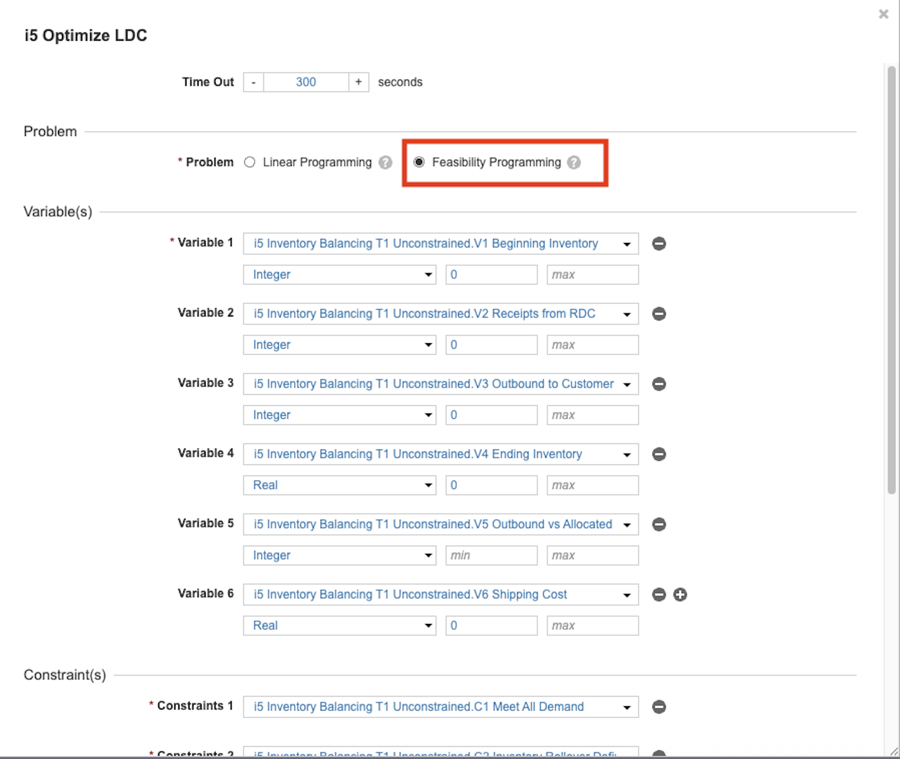
🔍 Disable some constraints - Create boolean switches to temporarily turn off certain constraints. This helpful trick lets you systematically identify which specific constraints are presenting challenges, bringing you one step closer to a solution.

• Create a model with disabled constraints, with a line item for each constraint. This simple step helps clarify the process and keeps your troubleshooting focused and organized.

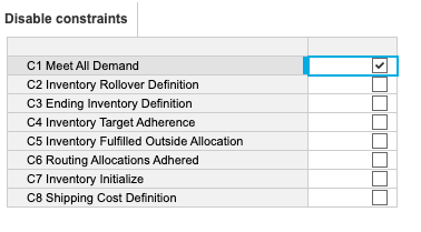
• Update your constraint formulas to: <disable constraint> OR <constraint>. For example: DisableConstraints.'C1 Meet All Demand' OR ('V3 Outbound to Customer' = Optimizer Demand by Customer). In this formula, if the disabled constraint switch is True, the overall statement is always satisfied, making the constraint inactive.  
  Explanation: Since all constraints must be True, if the boolean is True, the constraint is automatically satisfied, so the Optimizer ignores the equation. The Optimizer only checks the actual constraint if the boolean is False. This empowering method makes it easy to isolate which constraint is causing infeasibility, giving you control over your modeling process.
• Now you can disable the suspect constraint and run the optimization to check if the model has any feasible solution.

💡 Check solution feasibility - If you have a previous solution or a good guess, use the modeling interface to check which constraints are violated. This can quickly point you toward the problematic constraints.

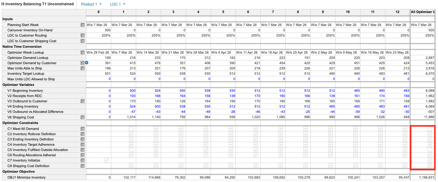
• All constraints must be satisfied for a solution to be feasible. In the summary, it's clear who is guilty. In this case, C1 Meet All Demand and C5 Inventory Fulfilled Outside Allocation are responsible for making this solution infeasible in the current model.
• Now that you’ve unmasked the main suspects. Dig into the constraint dimensions to pinpoint the source of trouble. In this case, you can see that the mystery leads straight to week 1 inputs.

Remember, every clue you uncover brings you closer to cracking the case 🕵️‍♂️

Getting Optimier logs helps to understand how to tweak the model to speed up the solving time. Workspace administrators can download the Anaplan Optimizer log via an API.
Links:
- Optimizer logs for debugging
-  https://anaplan.docs.apiary.io/#/reference/logging

Users can use Postman or perform this action directly in the browser. Step-by-step instructions on how to do this using the browser:
You will need 5 parameters:

• workspaceId,
• modelId,
• actionId,
• processId,
• and correlationId.

1️⃣  Authenticate into Anaplan and get workspaceId and modelId from the URL https://us1a.app.anaplan.com/…./workspaces/{workspaceId}/models/{modelId}/…

2️⃣ Getting actionId. https://us1a.app.anaplan.com/2/0/workspaces/{workspaceId}/models/{modelId}/actions

3️⃣ Getting correlationId. First, you would need to identify the process used to run the optimization. You can find it here https://us1a.app.anaplan.com/2/0/workspaces/{workspaceId}/models/{modelId}/processes . With processId you can now run https://us1a.app.anaplan.com/2/0/workspaces/{workspaceId}/models/{modelId}/processes/{processId}/tasks to get all the correlationIds for this process

4️⃣ Finally get the logs https://us1a.app.anaplan.com/2/0/models/{modelId}/optimizeActions/{actionId}/tasks/{correlationId}/solutionLogs

You should see something like this (with different values):

Optimize a model with 1011 rows, 936 columns and 2244 nonzeros

Model fingerprint: 0x7ef96434

Variable types: 390 continuous, 546 integer (0 binary)

Coefficient statistics:…

I hope this helps you to find the logs that you are looking for 😁